Our primary dataset came from Our World In Data's (OWID) COVID-19 Data. We decided to use this dataset as OWID curates their data from reputable sources including research from Johns Hopkins University (JHU), the United Nations, the World Bank, and many others. This dataset also has a plethora of variables available for analysis ranging from the number of confirmed cases and deaths on any given day to many other demographic variables such as human development indices and comorbidity factors.

With our first dataset, we looked at COVID deaths per million in individual countries as of June 8th, 2022. Using this “snapshot” dataset, we wanted to see if categorical variables (such as whether or not a country imposed a lockdown) were associated with COVID mortality rates. We also desired to know if quantitative but “static” type variables (such as diabetes prevalence in a country or that country’s population density) had any relationship with how each country fared in keeping COVID deaths down.

With our second dataset, we looked at COVID deaths per million over time. This time series data allowed us to see how different continuous variables were related to its COVID mortality rate. An important note with variables such as confirmed cases and deaths are that they are collected by date of report, rather than date of test/death. Therefore the number does not necessarily represent the actual number on a given date. This means that our data over time can show sudden changes (negative or positive) when a country corrects historical data, because it had previously under- or overestimated the number of cases/deaths.

One of the most interesting questions we hoped to answer with our chosen data was the effect of lockdowns – did they help individual countries to keep their COVID mortality rates down? We used an ANOVA model to test three different categories of lockdown – full, partial, and none.

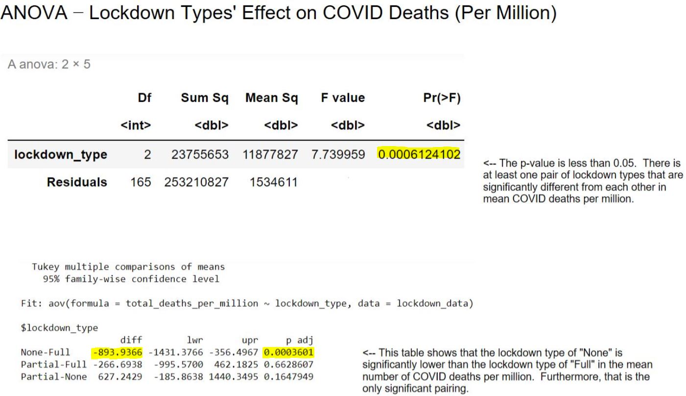
Interestingly, countries which employed a full lockdown had significantly higher COVID mortality rates (on average) than countries which had no lockdown whatsoever. This may be a counterintuitive result, but considering that countries with more COVID deaths may have been more motivated to try to use lockdowns to stem the number of deaths than countries which weren’t affected as much early on by the disease, the result is not entirely surprising.

Along with lockdown types, we were also interested in analyzing how different continents fared when it came to COVID mortality rates.

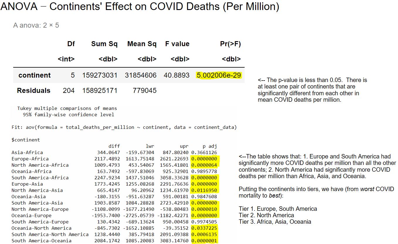
Based on the results of the model, it appears that countries in South America and Europe had the highest COVID mortality rates on average. North American countries had a lower mortality rate (on average) than South American and European countries, but a higher mortality rate (on average) than countries in Asia, Africa, and Oceania.

South America’s results may have been skewed by the country of Peru, which had a much higher rate of COVID deaths per million than was to be expected given its other variables (more on that later). The countries of Europe, on the other hand, may have been more afflicted with COVID mortality – especially early on in the pandemic – due to relative amounts of international travel in and out of Europe (although this was not something we could directly measure with our dataset).

There were many quantitative variables of interest in our “snapshot” dataset, and we divided these variables into two groups – one concerning what we called comorbidities, the other concerning what we named socioeconomic factors.

The comorbidity variables were cardiovascular death rate, diabetes prevalence, and the percentage of the population aged 65 or older.

For these variables, a preliminary multivariable linear model was constructed. Due to problems with the residual errors, two outliers were removed and a natural logarithm transformation of the response variable – namely, COVID deaths per million – was done in order to create the final model. The two outliers were Peru (with a much higher COVID mortality rate than the preliminary model suggested) and Japan (with a much lower COVID mortality rate than the preliminary model predicted).

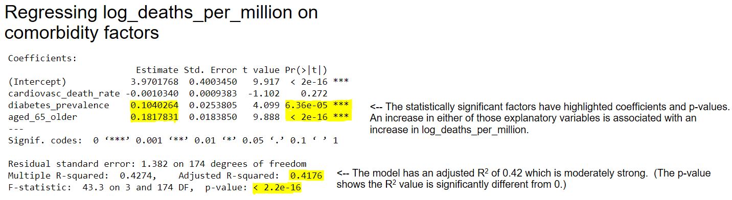
We found in the final model, which was moderately strong in explaining the variance in log-transformed COVID mortality rates, that the percentage of the population aged 65 or older and the prevalence of diabetes were both highly significant factors in the model. An increase in either of those explanatory variables was associated with an increase in the log-transformed COVID mortality rate. Contrastingly, cardiovascular death rate was not significant.

The socioeconomic variables were population density, life expectancy, and GDP per capita.

For the preliminary model using population density, life expectancy, and GDP per capita as factors, three outliers were removed and a natural logarithm transformation of the response variable (COVID deaths per million) was done due to problems with the residual errors. This became the final version of this model. The three outliers were Peru, Bulgaria, and Hungary – all with a higher COVID mortality rate than the preliminary model predicted.

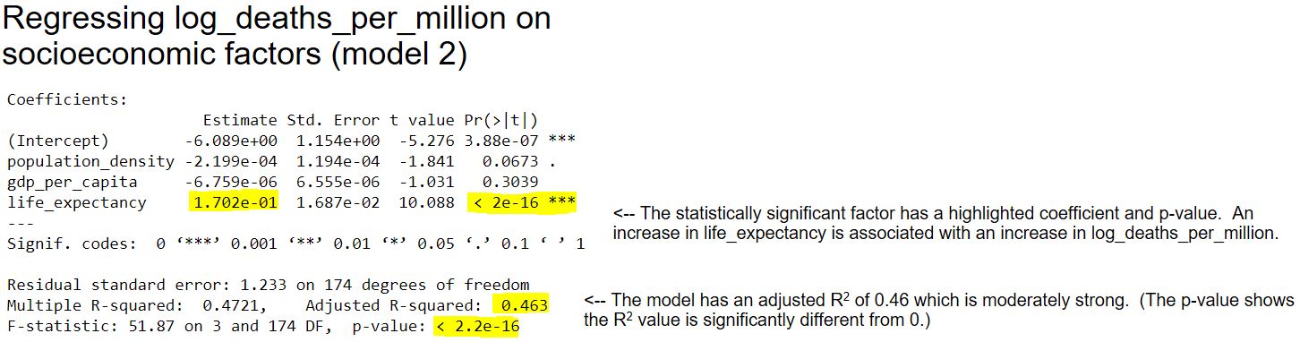
We found in the final model, which was moderately strong in explaining the variance in log-transformed COVID mortality rates, life expectancy was a highly significant factor in the model while population density was only a moderate factor in the model (0.05 < p < 0.1). An increase in life expectancy was associated with an increase in the log-transformed COVID mortality rate, while an increase in population density was associated with a decrease in the log-transformed COVID mortality rate. These results may be explained by the same reasoning given in the previous paragraph.

We also wanted to compare two models – namely, a socioeconomic factor model versus a comorbidity factor model – and their resultant R² values to see which model could better explain the COVID-19 mortality rate on specific continents.

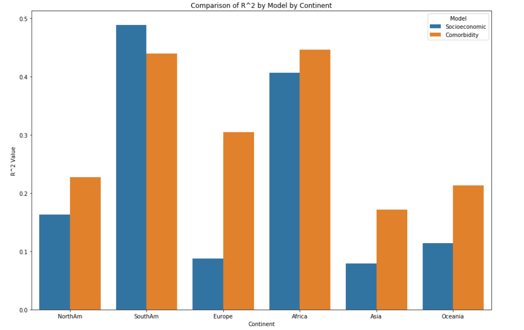
Both groupings of variables had low impact on the total COVID deaths per million for each individual continent as metrics such as R² were generally low – with the exception of South America and Africa, for which the R² values were moderate. The comorbidity features explained the highest percentage of variance for Africa (0.447) while the socioeconomic variables explained the highest percentage of variance for South America (0.489). Both sets of explanatory variables were insignificant to COVID deaths per million in Asia, with R² values of only around 0.08 for socioeconomic factors and 0.172 for comorbidity factors.

KMeans clustering analysis was performed on the snapshot dataset using socioeconomic, comorbidity and COVID totals variables as well as principal component analysis. The data was scaled using MinMaxScaler and the optimal number of clusters for the data in question was arrived at by use of a silhouette score analysis as well as an elbow chart.

For the socioeconomic data (life expectancy, GDP per capita, population density) the optimal number of clusters arrived at was 4. The data clustered nicely in an easy to interpret format, but the overall scatterplot was slightly crunched due to some outlier countries with higher life expectancy and population density than the rest.

For the comorbidity related data (population 65 years and older, cardiovascular death rate and diabetes prevalence), the optimal number of clusters arrived at was 7. The clusters make sense in that it is easy to see countries in Africa, Asia and Latin America with younger populations clustering together as well as North American and and northern European countries with older populations and higher comorbidity rates clustering together. It was interesting to see that many Pacific island nations have very high cardiovascular death rates and diabetes prevalence, and the clustering highlighted that fact.

Finally, a cluster analysis on the COVID related data (total deaths per million, total cases per million, total vaccinations per hundred) was probably the most useful out of the analyses conducted. The optimal number of clusters arrived at was actually 3 but we chose the second highest silhouette score at 8 clusters for visual effect and to call out outliers. The outliers Peru, Macedonia, Bulgaria, Hungary and Bosnia and Herzegovina were all encompassed in one cluster. It was also interesting to see how smaller countries, especially island nations with high vaccination rates, were able to keep their cases and deaths down.

Autoregressive Integrated Moving Average, or ARIMA, is a statistical analysis model that uses time series data to either better understand a data set or predict future trends. As dictated by our main questions, we are mainly interested in determining the primary factors, what we will call the exogenous variables, that drive mortality rates within our time-series data.

We chose our target variable for the model as new deaths smoothed per million. We hoped to show a relation between spikes in new deaths and changes in our exogenous variables. We used the smoothed data, which is a rolling seven day average because the variance in day to day data was very extreme. This also should help anomalies in the way different countries report their data from being too impactful.

For our exogenous variables, we looked at four variables: ‘people fully vaccinated per million’, ‘reproduction rate’ (real-time estimate of the effective reproduction rate of the virus), ‘icu patients per million’, and ‘hospital patients per million’.

People fully vaccinated is the exogenous variable we were most interested in. We hoped to show that as the number of people vaccinated increased that the number of deaths would decrease. We should see the inverse of this with Hospital and ICU patients. As their values increase we should see an increase in the number of new deaths.

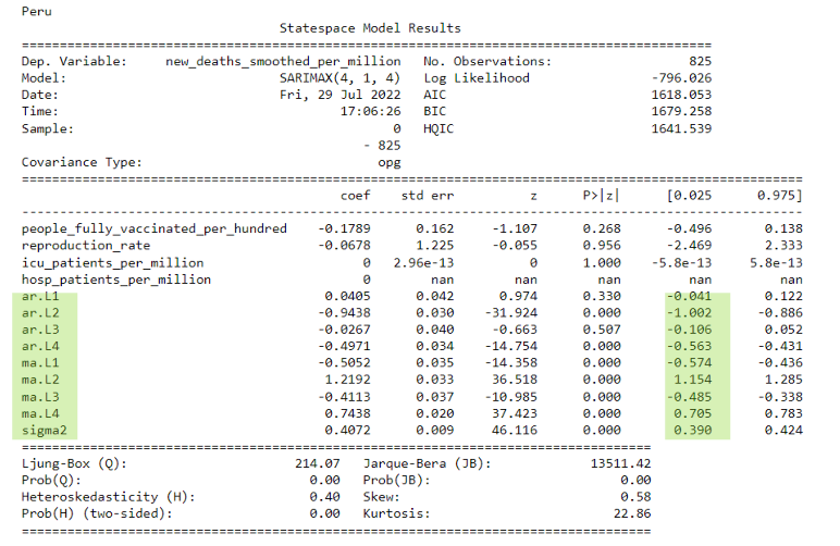
Pictured below are the ARIMA results for one of our outliers, Peru. The green areas are where we found significance due to these variables having p values of less than .05. As you can see, these are only the Autoregressive (AR) and Moving Average (MA) portions of the ARIMA model indicating that the recently passed results for a day have a higher effect on the next day than any of the exogenous variables we had entered.

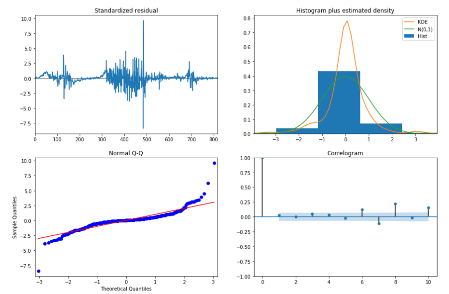
In the following slide, we see plot diagnostics for Peru's ARIMA Model. In the top left plot, the residual errors seem to fluctuate around a mean of zero but at random intervals have major spikes due to the introduction of new variants. The histogram plus density plot on the top right shows a slight skew towards the right with our data. This is also indicated by the Q-Q plot on the bottom left by the tail on the right skewing upwards. The ACF plot in the bottom right shows the residual errors are autocorrelated. Any autocorrelation indicates there is some pattern in the residual errors which are not explained in the model.

As shown in the prior ARIMA results summary, the p values of our exogenous variables were very high. This means that in relation to the other variables, in our case the auto regressor (AR) and moving average (MA) values, our exogenous variables were not as useful when predicting the daily new deaths of a country. The only significance as mentioned earlier were the AR and MA values which essentially indicates that data on any given date is more dependent on the results of previous days rather than any of our specific exogenous variables.

By mapping our coefficients against the total number of people fully vaccinated, we can see if there is a relation between them across all of the countries we made models for. Ideally, we would see that there is a negative correlation, which would show us that vaccinations had an impact overall. In our visualizations, we do not see any trends which does not mean that vaccinations are not effective, just not as important to our models as other variables. In our case, the AR and MA values are far more important in predicting the next day’s deaths.

Primary Factors Influencing COVID Mortality in Individual Countries

The primary factors we identified which are associated with COVID mortality rate in different countries are as follows: type of lockdown, life expectancy, continent, diabetes prevalence, and percentage of the population who are 65 years of age or older. For more details, please refer to the other slides that make up this website.

Interactions Among Primary Factors & Relative Strength of Models

In order to minimize interactions among the explanatory variables which might influence COVID mortality rate, we decided to use smaller models, each of which focused on one type of variable. We used two separate ANOVA models for our two chosen categorical variables, for example. As another example, we had a model focusing solely on comorbidity factors. Although smaller linear models tend to have smaller R2 values, we found the models to still be moderately strong. These smaller models are also easier to understand because they are appropriately focused.

It should be noted that we left certain variables out in our linear models because of their high correlations with other variables. We didn’t use a variable measuring the percentage of the population who are 70 years of age or older because it was highly correlated with the variable measuring the percentage of the population who are 65 years of age or older. We also left out a variable measuring human development index because of its high correlation with life expectancy, the latter variable being a much less complex variable (hence easier to understand).

Prescriptions for Possible Future Pandemics due to Airborne Virus

For many of the primary factors we found which are associated with higher COVID death rates, the countries involved may not be able to do much about them. For example, some countries have older populations, and there is little a country can do in the short term to mitigate that risk factor. However, there are at least two factors we analyzed which may be things countries can change in order to improve the worldwide result of another COVID-like pandemic. These factors are listed on the next two slides.

Diabetes prevalence. This was the only significant factor found in one of our linear models for which countries could undertake changes now in order to lower a future pandemic’s effect on mortality. Countries can promote healthier lifestyles (diet and exercise), and they can try to construct their healthcare systems so as to ensure all of their citizens have the ability to see doctors annually, pay for necessary pharmaceuticals, and so on.

Lockdowns. Our data showed that countries employing a full lockdown had higher mortality rates on average than countries which did not lock down. However, spikes in COVID mortality were mostly due to the appearance of variants, and research has shown that “the emergence of new, more contagious variants is being driven by uncontrolled transmission, not vaccines” (see SciTechDaily article). While individual countries might not be able to control the rise of variants in a COVID-like pandemic, it should be the goal of all countries to present a unified front in taking future pandemics seriously from the start.